At Nimbus Intelligence Academy we are trained to build a modern data stack including data warehousing, ELT processes and scheduled refreshing of data. Each trainee has set up a modern data stack in one day. This blog will showcase the approach of the project, where we highlight some key features of the data stack.
The blog is divided into multiple sections. Jump forward to any specific section by clicking on the link.
- Introduction
- Snowflake
- Snowflake set-up
- Database structure
- Warehouses and resource monitor
- Security
- Data loading
- Local files
- Fivetran
- Snowflake set-up
- dbt Cloud
- dbt set-up
- dbt environments
- dbt jobs
- Transformation
- Staging
- End tables
- dbt set-up
- Conclusion
Introduction
The «Modern Data Stack in One Day» project can be seen as a proof of concept for a client. At the end of the day, the client has a data stack in place with different sources and end tables that are ready to be used in business intelligence. The tools that we use to achieve this are Snowflake, Fivetran and dbt Cloud.
“We’re building a modern data stack in one day to convince a client to start a project with us. Treat this as a Proof of Concept.”
Snowflake is a cloud database platform where the data will be stored. Additionally, security policies and resource monitors are set-up within Snowflake. The data is loaded to Snowflake in two different ways; local csv files and a connection to the client database through Fivetran.
Once our data is loaded properly, we connect the Snowflake instance to dbt Cloud. Any further transformation of the raw data is done here. dbt also allows us to document the different steps in the transformation and, most importantly, use git for version control. In dbt Cloud we can schedule a job that rebuilds the data stack with a certain frequency. For this project we schedule to rebuild every morning to ensure that the latest data is present. After the job, we stage the data from the source. With SQL commands, the data is transformed into end tables. These tables should be ready for business use and thoroughly tested. With the use of dbt posthooks, we make sure that any security measures (e.g. row access policy) are in place for the end tables.
Snowflake
If you have read some other blogs of Nimbus Intelligence, you might know that we have a lot of knowledge on Snowflake. We use Snowflake intensively as a cloud database platform, because of its many unique features. Look through our other blogs to discover some of them!
Snowflake set-up
We set-up a Snowflake instance to host our data, and implement the structure of the modern data stack.
database structure
We start everything in Snowflake by creating the databases where our raw data and end tables are stored. The main principle is to have four databases:
- The RAW database stores the raw data.
- The DEVELOPMENT (DEV) database stores our initial transformed tables that dbt Cloud builds.
- The ACCEPTANCE (ACC) database is where our new transformations take place. Here we test the end models before we deploy them to the production environment.
- Last but not least, the PRODUCTION (PRD) database deploys the end models and final tables. This is the database that will be used for all the internal and external use from the business.
We will dive into more technical details, their structure and purpose later in the article.
warehouses and resource monitors
After creating the four databases we need to create the dedicated warehouses. Each warehouse will have a unique purpose and function. In general the amount of warehouses depends on the requirements of each project. Apart from the default warehouse that snowflake provides to every account (COMPUTE_WH), we created three more.
- The
FIVETRAN_WHwill be the dedicated warehouse for any loading done by Fivetran. This helps us to monitor usage specifically for this ELT process. - The
DEV_WHwill be the dedicated warehouse for all the data transformations the developers will do in dbt Cloud. The DEV_WH will handle every data transformation from the raw database to the dev, acc, and prd databases. - The
PRD_WHwill be the dedicated warehouse for any use of the end models in the prd database. It will be used by the analysts, team managers and in general roles that query the final tables.
The best practice to create warehouses is by using the SYSADMIN role in Snowflake, and then granting usage to the role that will use the warehouse. The code for every warehouse creation will be the same.
USE ROLE SYSADMIN;

CREATE OR REPLACE WAREHOUSE FIVETRAN_WH
WITH
    WAREHOUSE_SIZE = 'X-SMALL'
    AUTO_SUSPEND = 60
    AUTO_RESUME = TRUE
    INITIALLY_SUSPENDED=TRUE;
To help control costs and avoid unexpected credit usage caused by running warehouses, Snowflake provides resource monitors. We take advantage of that feature in order to keep track of credit spending for all our workloads in each warehouse. There are two ways to set up your resource monitor, either on the entire account level (every warehouse will follow that), or a specific set of individual warehouses.
USE ROLE ACCOUNTADMIN;
#since only the accountadmin role can set up resource monitors in an account.

CREATE OR REPLACE RESOURCE MONITOR FIVETRAN_RM
WITH
    credit_quota=100
    frequency = WEEKLY
    start_timestamp = IMMEDIATELY
    notify_users = (DIMITRIS, KRIS, ELOI, SEBASTIAN)
    triggers on 75 percent do notify
           on 95 percent do suspend
           on 100 percent do suspend_immediate;

ALTER WAREHOUSE FIVETRAN_WH SET RESOURCE_MONITOR = FIVETRAN_RM;
Now our warehouses are safe from over consuming credits. We have placed a limit on how much they can spend. We set up a notification in case 75% of the credit quota is spend. At 95% suspend the warehouse and on 100% suspend it immediately.
security
network policy
When it comes to security Snowflake has another great feature where users can set up a Network Policy. This was also a requirement of the project. We had to set up a Network Policy that would allow users to login to Snowflake only from specific locations. One from our individual IP addresses and also from the office’s. To set up the Network policy we used the following code:
USE ROLE SECURITYADMIN;
#we use the recommended from snowflake role to set up the network policy

CREATE OR REPLACE NETWORK POLICY access_policy_ip
   ALLOWED_IP_LIST = ('<personal_ip_address>', '<office_ip_address>')
   COMMENT = 'This network policy holds the ip address of the developer/engineer and the clients ip address';
To see if the network policy is in place and working as expected we run the following command:
DESC NETWORK POLICY access_policy_ip;
Users and roles
At this point, the databases are in place, the dedicated warehouses have been created and waiting to run our workloads, our resource monitors are seated on the warehouses to keep our credit spending under control and our network policy is in situ to allow users login from certain ip locations. However, we miss a major part of our project. The creation of certain users and roles.
The structure of the users and roles the PoC requires, based also on the client’s requests is the following:
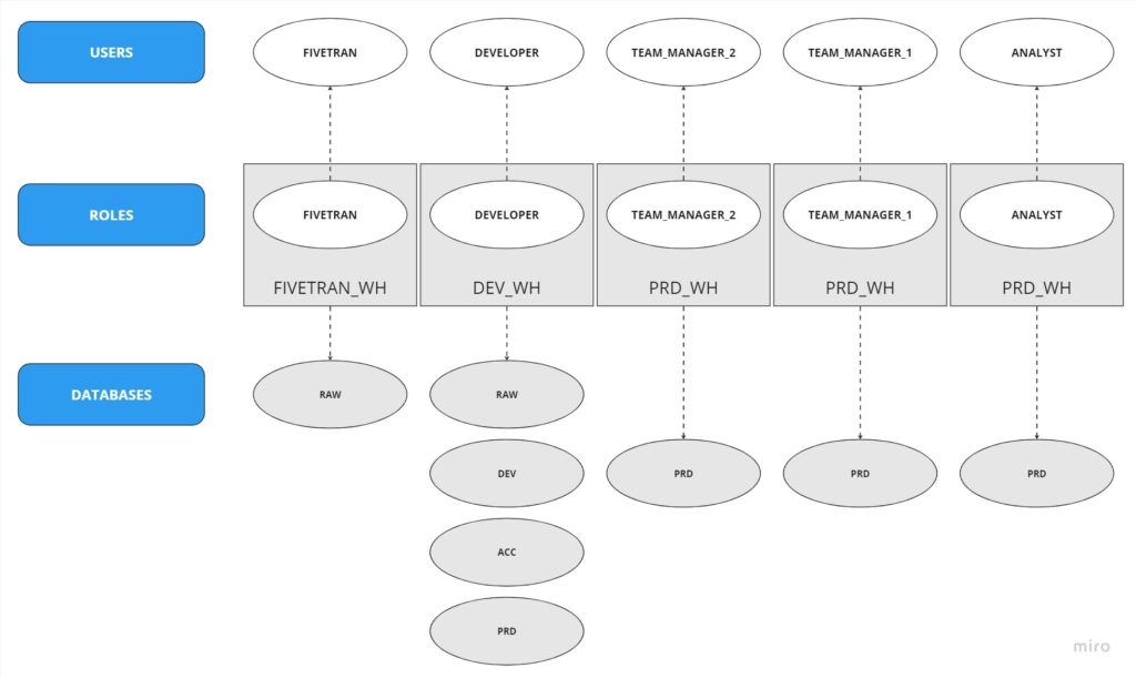
As we see in the above diagram the structure of our roles and users is quite intuitive. However, someone can easily get lost especially when you have multiple users that have been assigned multiple roles, while working on different warehouses.
For this project we need to create 5 different users with their corresponding roles. FIVETRAN user that will have the FIVETRAN role and will have access only to the RAW database and will use the FIVETRAN_WH. The DEVELOPER user will have the DEVELOPER role and will run all the transformations in dbt, will work on the DEV_WH and will have access to all the databases. The Team Managers 1, 2 and the ANALYST users. They will be granted the corresponding roles and will have access only in the PRD database where our end models and final tables exist. Last but not least, they will make use of the PRD_WH.
The code for creating the users follows more or less the same structure for each user creation:
USE ROLE USERADMIN;
# The default role Snowflake suggests to create new users

CREATE USER IF NOT EXISTS FIVETRAN_USER
   password = '<the password you want to set>'
   default_role = 'FIVETRAN'
   default_warehouse = 'FIVETRAN_WH';

CREATE OR REPLACE ROLE FIVETRAN;

GRANT ROLE FIVETRAN TO USER FIVETRAN_USER;
#You need to grant the role to the specific user. The rest of the roles go accordingly.
privileges
Snowflake documentation provides many options on granting privileges. As Nimbus Intelligence we always provide the minimum required privileges to each role to maximise our system’s security. The overall structure of the privileges is divided in four parts:
- USAGE on the dedicated warehouses, for all users to their corresponding warehouse
- USAGE on the databases each role requires to have
- USAGE or CREATE Schemas in/on database, based on the characteristics each role has
- USAGE on future Schemas in the database for the DEVELOPER role.
For this project an example of granting privileges to the above mentioned roles is the following:
GRANT USAGE ON WAREHOUSE FIVETRAN_WH TO ROLE FIVETRAN;
#Usage on the dedicated warehouses will be accordingly with the rest of the roles.

GRANT USAGE ON DATABASE RAW TO ROLE FIVETRAN;
#usage on the rest of the databases and the rest of the roles will be accordingly as well.

GRANT CREATE SCHEMA ON DATABASE RAW TO ROLE FIVETRAN
#In order for the FIVETRAN user to import the raw data from the Fivetran connection it needs the create schema on database privilege.

GRANT USAGE ON FUTURE SCHEMAS IN DATABASE PRD TO ROLE DEVELOPER;
#Provide the developer with the necessary privilege to create new schemas in the databases in order to let dbt run the commands and build the tables.
Data loading
For the modern data stack we retrieved the data from two sources as mentioned earlier.
local files
The data provider delivered to us a number of files manually from a shared storage platform, in this case Google drive. Subsequently, we retrieved 5 tables, employee_info_1-4 and the employees table. These tables were loaded into Snowflake through three steps. Firstly, we created the two tables. Secondly, we staged the correct files through SnowSQL. Lastly, we run the two COPY INTO statements shown below.
#Employees table
COPY INTO employees FROM @%employees/employees.csv
FILE_FORMAT = (TYPE = CSV
                SKIP_HEADER=1
                DATE_FORMAT = 'DD-MM-YYYY');

#Employee info tables
COPY INTO employee_info FROM @%employee_info
FILE_FORMAT = (TYPE = CSV
                SKIP_HEADER=1);
For a more detailed explanation of loading local data into Snowflake, check out this blog of our Italian colleague Mario. Another way to upload data is to create named stages directly in Snowsight. In May 2023, Snowflake released a new feature where users can manually upload files from their Snowsight with one limitation however, the files must be smaller than 50MB. The Employee_info_1-4 have in total 8 KB so we upload them through our Snowsight. Snowflake takes care of the file formats and the stage. This article describes this method in more detail.
raw data
Now our Snowflake instance has two tables in the RAW database. We show a preview of the tables below.
| ID | FIRST_NAME | LAST_NAME |
| 201 | Camille | Matej |
| 202 | Roxanne | England |
| 203 | Kristien | Bradick |
| … | … | … |
| EMPLOYEE_ID | DATE1 | DATE2 | TEAM |
| 1 | 2010-04-17 | 2010-11-20 | 7 |
| 2 | 2009-08-09 | 9999-12-30 | 6 |
| 3 | 2023-03-22 | 2023-04-28 | 2 |
| … | … | … | … |
fivetran
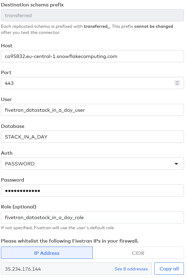
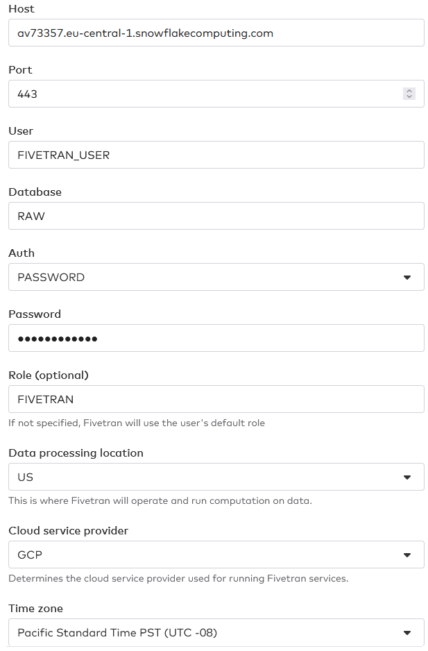
For the second method of retrieving our raw data we set-up a connection with Fivetran. The Fivetran set-up is pretty simple. We must provide Fivetran with the account and database where it needs to get the data from. Moreover, Fivetran will access the data as if it was a normal Snowflake user. Therefore, we must initially create a role, user and password for Fivetran. Fivetran will use these to read and load data from one account to another. For the source database, it will need reading privileges, while for the destination account (the one that we must set up in this case) it will need to also have CREATE SCHEMA privileges. Of course, Fivetran needs access to a warehouse as well. The queries to move the data around cannot run without a warehouse.
raw data
Once the connection is made, we are able to view and select the schemas and tables to be transferred and the data will start to synchronise. As a result, we will be able to see two new schemas with five tables in total in our RAW database. Fivetran automatically generates two of these tables which contain information and logs about the data transference. The other three are the nation, region and customer tables that the data provider has transferred to us.
| N_NATIONKEY | N_REGIONKEY | N_NAME | N_COMMENT |
| 23 | 3 | UNITED KINGDOM | Some comment |
| 3 | 1 | CANADA | Comment here |
| 9 | 2 | INDONESIA | This is now |
| … | … | … | … |
| R_REGIONKEY | R_COMMENT | R_NAME |
| 1 | What now | AMERICA |
| 2 | Some information | ASIA |
| 4 | Some line filler | MIDDLE EAST |
| … | … | … |
| C_ACCTBAL | C_NATIONKEY | C_ADDRESS | C_CUSTKEY | C_COMMENT | C_MKTSEGMENT | C_PHONE | C_NAME |
| 8’345.65 | 17 | Tiger Str. | 34 | Good customer | MACHINERY | 01234 | Cust#34 |
| 2’455.30 | 9 | Elephant Way. | 6745 | Spends to much | AUTOMOBILE | 23456 | Cust#6745 |
| 5’324.10 | 17 | Fish Str. | 4565 | Pay attention | FURNITURE | 34567 | Cust#4565 |
| … | … | … | … | … | … | … | … |
dbt Cloud
Nimbus Intelligence works with dbt Cloud, but what is dbt? One of our team members has written a blog about dbt and machine learning, where he also answers this question.
«dbt, or Data Build Tool, is an open-source command-line tool. Specifically, dbt allows users to build, test, and deploy data pipelines with ease. Many of the tasks associated with managing data pipelines can be automated using dbt.»
Sebastian Wiesner
dbt Cloud is the user interface of dbt that can be opened in any browser and does not require any command-line set-up. We highly recommend it for building a modern data stack because it has version control, easy documentation and insight into the lineage of the data stack.
dbt set-up
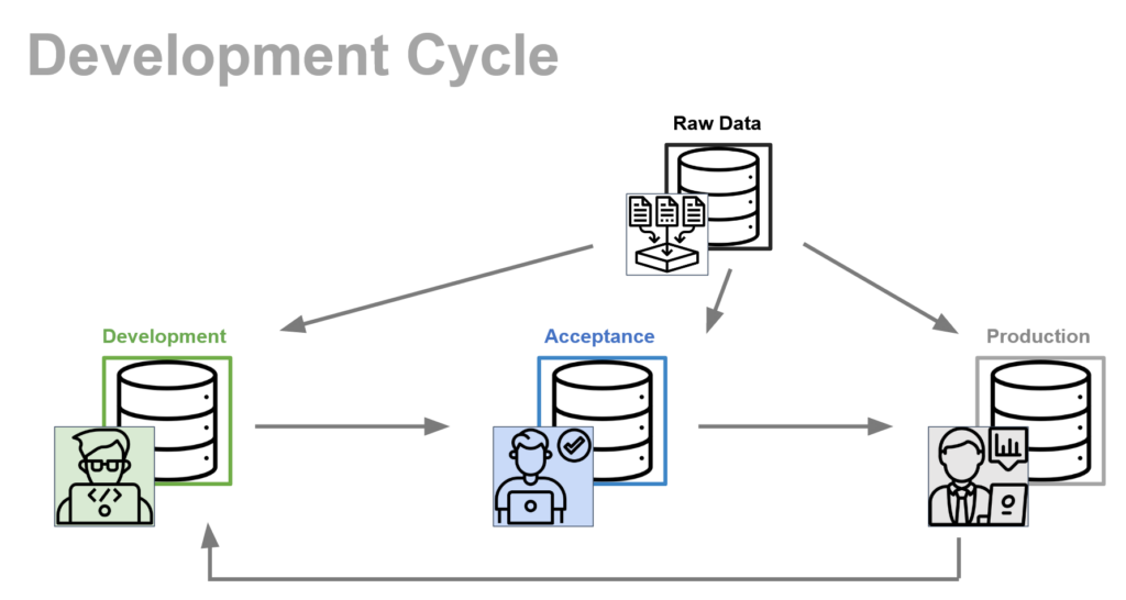
Initially, we have already mentioned that we split our work in three different databases, DEV (for development), ACC (for acceptance) and PRD (for production). The idea is to completely isolate the Production database from any harm during development of new features.
The main idea is the following:
- Developers build and test new features in the DEV database.
- Once the features have been built and tested in the development environment, which is unique for each developer, the changes are introduced in the Acceptance environment, i.e., the ACC database.
- Finally, once the changes in Acceptance have been properly tested and everything is working properly, the changes can be merged from Acceptance to Production.
During development, developers work in an individually isolated environment so that changes of a developer do not affect the results of other developers. Since all developers use the same development database, the compartmentalization of environments happens through schemas prefixed by some unique developer code, for instance, dbt_{developer_initials}_{schema_name}.
However, in Acceptance, we must make sure that all changes can coexist together without creating conflicts, since we want to simulate as closely as possible what we will have in Production. Therefore, in this environment we will not have distinctions between different developers and the schema structure in the ACC database will have to share exactly the same structure as what is found in PRD.
The final merging of Acceptance to Production, once everything has been tested out, will be fairly simple, since Acceptance is basically the Production environment with some extra changes. Overall, we set-up the developing cycle for the modern data stack as in the following picture.
dbt environments
But, how do we make this happen in dbt? Well, in dbt, we can set up different environments. Each of these environments connects to a different database. We create Jobs that build the contents of said databases according to the current state of a determined branch in our git repository. Therefore, we can make three different rules for our three different environments.
| Environment | Follows git branch | Takes data from | Builds to database |
| Development | Branch with new feature | RAW | DEV |
| Acceptance | acceptance | RAW | ACC |
| Production | main | RAW | PRD |
For a developer, the working cycle is pretty simple.
- Create a new branch in Git starting from main.
- Develop and test new changes in the new branch in her own development schema
- Merge the new branch to the acceptance branch
- Build and test the changes in the ACC database
- Repeat until push to production
All developers will follow this until the end of a sprint or the launch time of a new release. In that moment, the acceptance branch is merged to the main branch and the following dbt build will introduce the new changes to the PRD database, available for the rest of the company to see.
Ideally, and for a single developer, the GitHub graph network should look something like the image below.
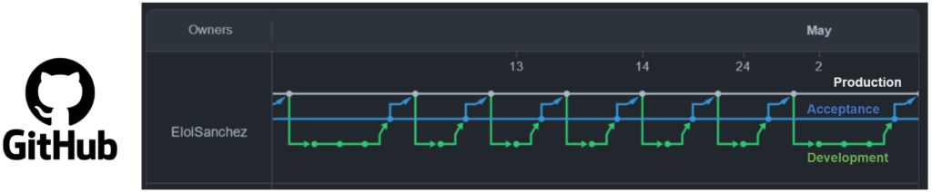
Notice that the only pushes to production come from the acceptance branch, and all development branches initially come from the production branch. The changes take place in development and then are merged to acceptance finally reaching production.
dbt jobs
Now that we understand the three different environments in dbt we can go into the orchestration of our Snowflake databases. How and when do we introduce new data to production? How and how often do we test our acceptance environment? dbt Cloud manages this using Jobs.
Jobs are (partial) rebuilds of the Snowflake databases. Unless the build includes incremental models, every time dbt runs a job, it will delete all data from the database and rebuild it from scratch, introducing in this new build the new data from the raw sources. This process, especially for larger companies with huge amounts of data, is an expensive process. Therefore, careful planning and scheduling is of the utmost importance to reach a balance between data latency and freshness and reducing expenses.
For most cases and companies, a daily rebuild of the PRD database just before the working day begins should be enough. This ensures that the analysts will get all the fresh data until the previous day.
As for the ACC and DEV databases, they should be run as needed. Developers should make sure that they do not make full rebuilds unless they are needed. Partial rebuilds including the models that are being affected by the changes should be enough. Once the new changes reach acceptance, a proper full rebuild should probably be considered to make sure that the changes are working as expected outside of the developers controlled environment.
| Database | Build frequency | Build size |
| DEV | As developer needs | Partial, affected models with limits in the SQL queries |
| ACC | When new changes must be tested | Full rebuild |
| PRD | Periodically to refresh data for analysts | Full rebuild |
Transformation
The transformation from raw data to end tables for our modern data stack is solely done in dbt Cloud.
staging
The data transformation starts in dbt in the staging section. In this step, we will create the staging models that will get the data from the source tables in the RAW database. During this process, we will avoid performing any major transformations to the data except for minor changes such as column renaming. The idea is that we get an almost identical copy of the raw data in our target database, ready to be used by the intermediate and final tables.
- Employee_info
In this case, we gather all information as was in the database. We do not change anything. - Employees
We rename the columns date1 and date2 to start_date and end_date respectively. - Customers, regions and nations
In the raw data, all column names are preceded by the first letter of the table name, (i.e.c_name,c_acctbalorr_regionkey). We can choose here to rename the columns if we would like to in case we need to follow any company standards.
End Tables
The «Modern Data Stack in One Day» project focused on creating a complete data stack using the tools Fivetran, Snowflake and dbt. This chapter will look in detail at the final tables that were delivered as the main results of the project using dbt. The chapter introduces the minimum viable products.
All final tables have different tests to ensure that the data is consistent. These include classic dbt tests such as not_null and unique on the respective ID columns of the tables. Additional tests used are explained in more detail in the individual sections.
The dbt materialization determines how dbt builds and stores the output of a model or table. There are three main types of materializations: table, view, and incremental. Different developers in the project may have chosen different materializations based on the specific requirements of their models or tables. The choice of materialization depends on factors such as data volatility, performance needs, and the intended use case, allowing developers to tailor their approach to the unique characteristics of their data and project goals.
Table employees
One of the final tables created is «employees«. The data for this table was extracted from a single CSV file. To keep the data standardised, the date columns were transformed into datetimes and renamed. In addition, a test was carried out to ensure that the teams were numbered in a valid range from 1 to 10. This ensures consistency and accuracy of the data, which is crucial for later analyses. For this test the dbt package dbt_utils was used. Using the “accepted_range” macro it was possible to test if only values between 1 and 10 were inserted into the table.
Table ex_employees_days_on_contract
Another important end table is «ex_employees_days_on_contract«. This table is based on the «employees» table and calculates the number of days of service per employee ID. It excludes employees with an active contract, identifying active contracts by a specific expiry date. By calculating the days of service, we gain valuable insight into the employees’ past length of employment.
Table employees_active_per_month
The table «employees_active_per_month» provides a comprehensive overview of the count of employees with active contracts for each month within a specified year, taking into account active contracts until December 31, 2023. This table serves as a valuable resource for analyzing trends in employee employment over time, offering crucial insights for effective workforce planning.
Table customer
The «customer» table was enriched with additional information on nations and regions. Furthermore, to ensure better organization, this table has been stored in a separate schema. By incorporating geographical information into it, we can conduct geographical analyses and gain a deeper understanding of the relationships between customers and their locations. In order to achieve this, multiple tables were joined together to gather the necessary information. Through the utilization of Common Table Expressions (CTEs), the structure of the joins becomes clear and complete. Consequently, using CTEs enables other developers to swiftly grasp an overview of the resulting table.
Table intermediate_table
To facilitate more comprehensive data analysis, an additional schema called «intermediate_table» was established. Within this schema, a date dimension was created utilizing the dbt_utils package and Dataspine macros. This dimension incorporates quarter, month, and week numbers, thereby offering a structured time series perspective of the data. Consequently, it simplifies the examination of trends across various time levels and enables more precise time-based analysis.
Table manager_table
By utilizing dbt seed, a table named «manager_table» was successfully generated. Adhering to the roles in Snowflake, a dbt seed table was created to contain pertinent information such as the username and corresponding team number of each manager. This information was directly incorporated into the csv files within dbt, ensuring seamless integration into the manager_table.
Row-level access policy
As part of the modern data stack in one day project, we implemented a row-level access policy to ensure data security. This chapter looks in detail at the different aspects of access policies.
Policy steering
Firstly, we created a special data source called «manager_table» as a starting point for the access policies. Additionally, this table contains information about the managers in the organisation and serves as the basis for the access restrictions. By utilizing this table as a single source of truth, the implemented policies ensure that only a specific team manager can view its own team members.
Policy creation
Secondly, to enforce strict data access control within the employee table, we created a row level access policy using the capabilities of a post-hook. This is a feature of dbt that allows you to execute any SQL command as soon as the model is build.
Using a post-hook, we defined a policy that ensures only the corresponding team manager has access to view the team members from their specific team within the employee table. This policy was implemented to maintain data privacy and security while providing the necessary visibility to team managers. The SQL is found in a separate macro that creates or replaces the policy.
#Create or replace RLA policy
CREATE OR REPLACE ROW ACCESS POLICY {{database}}.{{ schema }}.rla_employees
    AS (team int) RETURNS BOOLEAN ->
        'ACCOUNTADMIN' = CURRENT_ROLE()
        OR 'DEVELOPER' = CURRENT_ROLE()
        OR EXISTS (
                SELECT * FROM {{ database }}.{{ seed_schema }}.manager_table
                WHERE 1=1
                    AND 'TEAM_MANAGER' = CURRENT_ROLE()
                    AND username = CURRENT_USER()
                    AND team = manager_table.manager_of_team
         )
With the use of macros and post-hooks, the policy creation process was straightforward. We leveraged the functionalities of dbt Cloud to define the policy rules based on the manager-team relationship. By specifying the appropriate filters and conditions using SQL, we were able to restrict access to only the relevant data.
Policy application
We employ a second post-hook to seamlessly apply the access policy to the employee table subsequent to its creation. The post-hook script encompassed the essential SQL statements required to associate the access policy with the table. By following this procedure, we guaranteed the enforcement of the policy when generating the employee table using dbt.
#Applying RLA policy
ALTER VIEW {{model}} ADD ROW ACCESS POLICY {{database}}.{{schema}}.rla_employees ON ('team')
By incorporating dbt post-hooks into our data pipeline, we achieved a streamlined and automated process of applying the access policy. The post-hook executed the necessary SQL commands, linking the policy to the table, and thus ensuring the appropriate data access restrictions were in place.
Conclusion
In this blog we have taken you through the Nimbus Intelligence approach of setting up a modern data stack in one day. We have used our favorite tools to build the data stack, Snowflake and dbt Cloud. Furthermore, we focused on a robust and secure set-up that could serve as a proof of concept for a client. Has this blog peaked your interest in modern data stacks? Feel free to contact us!