It is fair to state that, nowadays, we often happen to hear that data is the new gold. If it is true that potentially the real treasure possessed by companies is represented by data, then entrepreneurs must be aware whether they own a vault full of bullion bars or a mine where to dig nuggets out of the mud. Indeed, even more importantly than the total amount of data of which firms dispose, it is how they are stored and subsequently used that impacts on the company’s growth. A rule of thumb to follow to achieve success is to avoid being one of those companies that – in the words of Robert Waterman in In Search of Excellence – are “data rich but information poor”.

The big challenge for companies today then consists in building their business having as two of the fundamental pillars a clean and structured way of storing data and a skilled workforce able to process them. In the following lines, we will try to provide a brief view on two concepts that could help transforming huge amount of data into valid information, focusing on at which level they apply to and on how interconnected they are.

Let’s talk about data normalization and table joins!

What is Data Normalization?

As just stated, one of the goals of good database design is to eliminate unnecessary and duplicate data. The term data normalization, or database normalization, identifies the whole set of rules and formalism involved in the process of creating and organizing the entities of a database in such a way to cut down data redundancy, i.e. duplicate data.

In other words, data normalization is the modality to ensure the unique and logical storage of every field and record whithin a database.

A normalized database will thus be lighter and more efficient that an unnormalized one: as a fact, avoiding redundancies reduces the need of database storage space. Moreover, data normalization turns the database into a structure more compliant to the relational model, increasing its overall performances: troubleshooting and maintenance become easier, queries are simplified and all the applications and processes of a company that run on some data contained in the database are sped up. As you might have already guessed, this implies gaining resources and saving lots of money on the long run!

It is a simple concept: data normalization is all about the specific criteria that must be followed when setting up an organized database, but putting them into practice is more complex than it might look. What do they actually say?

Data Normalization Levels

The first rule of our data normalization club, or 1st Normal Form (1NF), states that in each table (entity) of our database there should be no repeating columns (attributes), that each column should contain a single value of a specified type per row (record) and that each row should result in a set of single values identifiable through a unique label (key).

The second rule (2NF) asks us to create relationships, based on keys, between the different entities in order to be able to later put them in connection.

Finally, the third rule (3NF) – which is also the level at which the majority of transactional databases work and process their data – aims to directly reduce redundancy by including in a table only those attributes that directly relate to the entity.

Let’s look at an example to help us visualise what Data Normalization means:

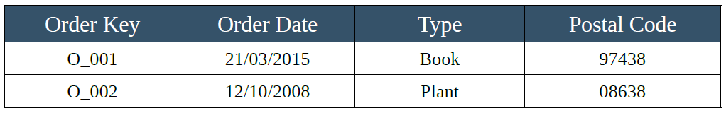
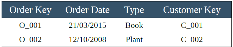
We can pretend to be hired by a shipping company whose database has records that are stored in a single entity of this type:

We immediately realize that this database is not normalized. Data are stored in a single table, there’s redundancy and it’s hard to understand which information classify the customer and which the shipments from our company. Moreover, if we imagine that one of our customer could place a new order, we would burden the table by inserting again his/her information. We cannot stand this system any longer, it’s time to act!

First Data Normalization level:

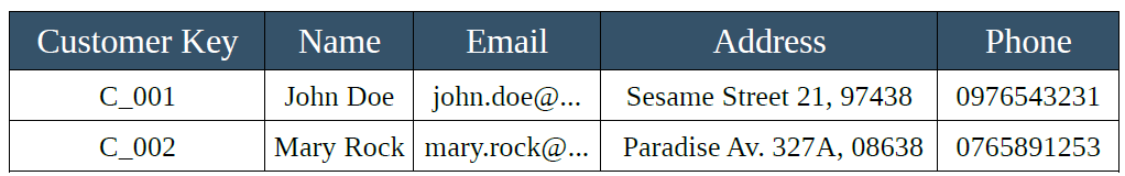
1NF tells us to split tables and to generate a unique key that will help us identify each row when needed. We decide to create a table for the customers and one for the orders:

The database now consists of more entities, each with its own attributes and unique key, that from now on will start calling primary key.

Second Data Normalization level:

At this point though, the tables appear to be completely unlinked. Following the 2NF, we generate a connection between them by adding in the order table a field that will allow us in the future to understand which customer has placed a particular order:

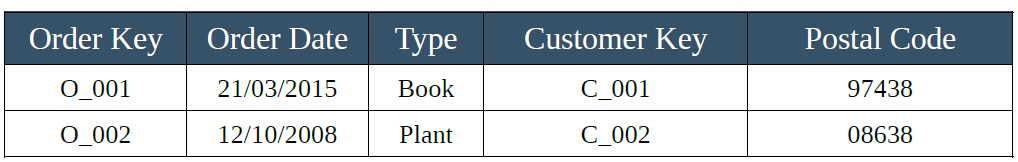
The easiest way to generate this connection is represented by the customer key, a specific identifier that, once read, allows us to retrieve every other information concerning that customer by simply consulting its “parent” table.
When the primary key of a parent table is inserted into a second table to create a connection between the two entities, it takes the name of foreign key. In this case then, our customer table only has a primary key (customer key) and our order table has a primary key (order key) and a foreign key (customer key).

Third Data Normalization level:

The last step is to apply the rule to reach the 3NF level: we have to remove redundancy. We notice that the order table still states the postal code at which to ship the orders. This information not only depends on the customer and not on the order, but is also already contained in the customer table. To fix it, we operate as it follows:

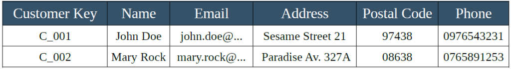
The entities in our database are now normalized, clean and will allow us to update our customer list and order history without overloading our system with useless information. It will also be possible to associate multiple orders to a single customer by recalling its customer key in the order table. The whole transactional system will thank us!

To wrap it up:

The best practices to reach the 3rd Normal Form (3NF) can be briefly summarized as:

• Split data into multiple entities (tables) so that each piece of information is represented only once and labelled with its own ID (key).
• Each database must have only one primary key.
• All the non-primary keys must be fully dependent on the primary key.
• Remove all transitory dependencies and avoid redundancy.

Table Joins in Normalized Databases

It is now time to address the second point of this guide: once a skilled unit of data engineers has set up an organized database minding data normalization, it comes the turn of the company’s analytics engineers. These figures are able to query, retrieve and elaborate the data stored inside the tables created by their fellow colleagues.

Their job is indeed to transform data into information that can generate surplus value for the company. Simply put: their task consists in merging, modifying and executing mathematical or statistical inferences on the data to help decisions in marketing, development, growth, client management or sales.

In this perspective, connecting records from different entities comes in handy. Essentially every database can be prompted through SQL-based platforms and the conjunction operation (JOIN) allows to link together information distributed in multiple tables through the association between the aforementioned keys.

At the risk of appearing tedious, let’s quickly reiterate the key types previously introduced:

• Primary key: Original key type. According to the 1st Normal Form, there can’t be more than one primary key per table, and all the fields must be directly and fully dependent on it.
• Foreign key: Secondary key used to relate a table to a parent table in which this key figures as the primary key.

Types of Table Joins

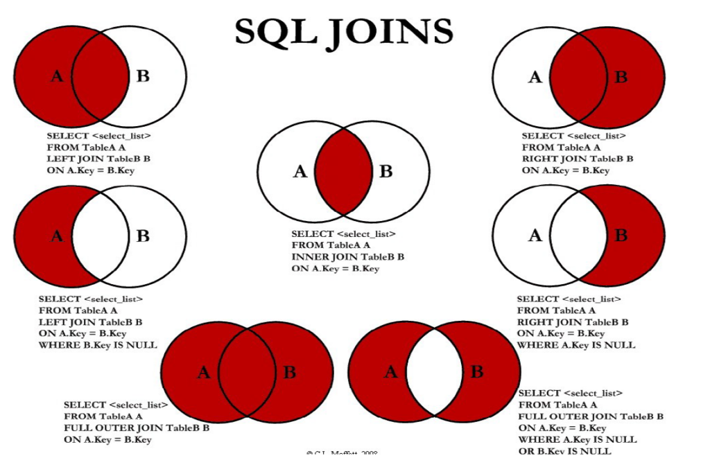
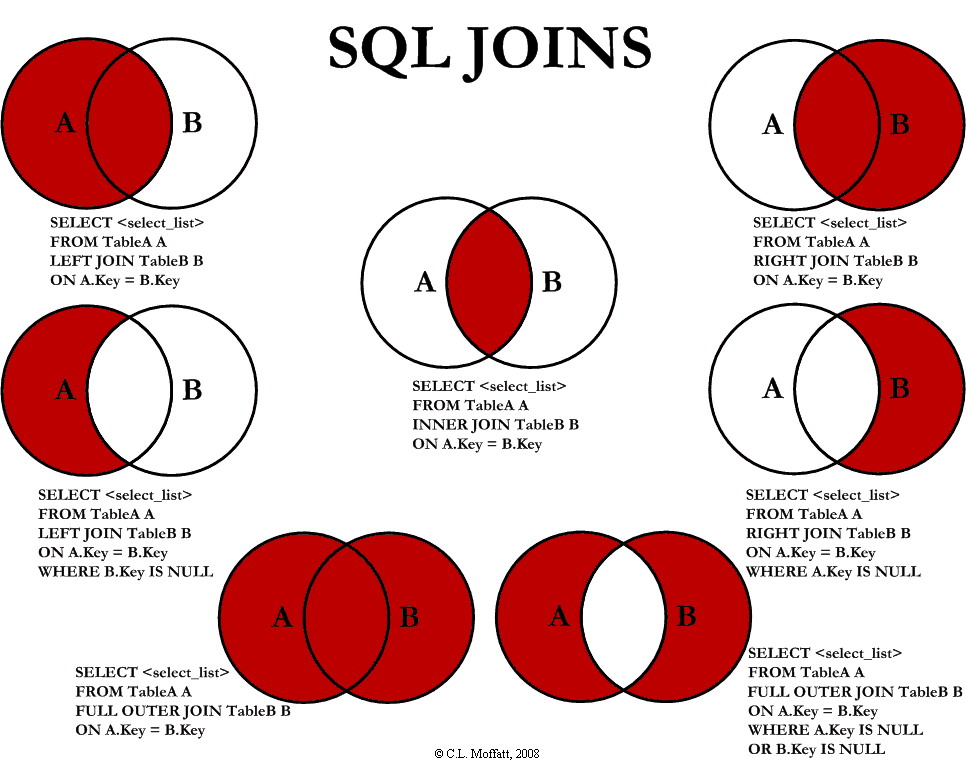
Linking the keys of two tables, it is possible to then create different joins according to the type of preferred intersection between the two tables. What types of joins exist?

Inner Join: An inner join connects two tables but only return matching rows in both tables.
Left Join: A left join is one in which all records from the left table and all matching records from the right table are returned.
Right Join: A right join is one in which all records in the right table and all matching records in the left table are returned.
Full Outer Join: A full join uses left join and right join, and returns all rows from
both tables in the output.

It is important to mention that, if no value is found, a NULL value will be returned in the columns appended to the original table. Equally important, the condition of a NULL key will return only the data that do not belong to the intersection of the two tables.

The syntax is pretty straightforward and can be observed in the picture above. The utility of this operator is that there is basically no limit to the number of tables that can be joined together, as long as they dispose of the right keys to establish a link.
For a deeper understanding of JOIN, please check out our blog!

Let’s put this knowledge on Table Joins into practice:

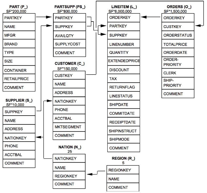
Through this Snowflake sample database it is possible to work on the data relative to the supply chain of a fictional firm. One interesting task could be for example, to find out what is the average discount applied to line items in orders placed by customers from each region.

To obtain this result, it is necessary to find information that lay in two different tables (Lineitem and Region) that are not directly connectable to each other. However, the two tables can still be linked together considering that the information relative to the production line, the customers that placed an order and which region are they from are found in other tables that can be used as a bridge:

Lineitem – Orders – Customer – Nation – Region

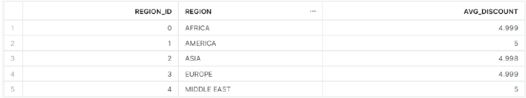
The final elements that we are interested in are the attributes of the different regions (their ID and their names) and the average discount – expressed as a percentage – of which each region benefits from. To return only these values it had been necessary to group the different orders per region before checking the discounts applied to them; again, this operation was performed through a “multiple join sequence” that put the two interesting tables in contact!

SELECT DISTINCT R_Regionkey                                          AS Region_ID
              , R_Name                                               AS Region
    	      , 100*AVG(L_Discount) OVER(PARTITION BY Region_ID)     AS Avg_Discount
         
FROM Lineitem
INNER JOIN Orders
ON Lineitem.L_Orderkey = Orders.O_Orderkey
INNER JOIN Customer
ON Orders.O_Custkey = Customer.C_Custkey
INNER JOIN Nation
ON Customer.C_Nationkey = Nation.N_Nationkey
INNER JOIN Region
ON Nation.N_Regionkey = Region.R_Regionkey
WHERE 1 = 1
ORDER BY Region_ID;

That’s it for this introductory dive into data normalization and data extrapolation through table joins!

Have questions about merging data? Be sure to check our blog.