Let’s talk about partitions!
The desire to partition large amounts of data organized in large tables within data warehouses stems from the need for better performance and better scalability, ways to achieve this are micro-partitions and clustering.
Partitioning traditionally follows a static approach whereby these tables are divided into smaller tables organized according to criteria (List Partition, Range Partition, Hash Partition).
This approach has positive aspects compared to managing a single large table but still has critical issues.
Issues are related to the consumption of computational resources, to maintenance and also the characteristics of the data that may not be organizable homogeneously and in partitions of similar numerosity, so the result may not be particularly beneficial.
How, then, to have a form of partitioning that is as advantageous as static partitioning but does not have the same critical issues?
Snowflake answered this question with micro-partitioning!
Let’s see what it consists of:
Let’s start with the atomic unit of micro-partitioning: all tables in Snowflake are automatically divided into micro-partitions with sizes ranging from 50MB to 500MB ( N.B that even the lower limit represents a constraint, we will see later when we talk about how new data is inserted) of uncompressed data.
Groups of rows in the tables are mapped into columnar form micro-partitions this allows for very high granularity. This organization ensures that all row elements belong to the same micro-partition.
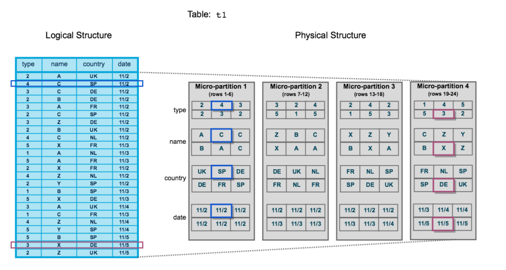
Each micro-partitions is characterized by some metadata:
– range of values present
– number of distinct values
– other properties for query optimization
But what are the real advantages of this approach?
– Micro-partitions are automatically generated so there is no need for any kind of user maintenance or explicit declaration.
– The small size ensures reduced granularity and fast and efficient execution of DML family commands.
– The overlap of the micro-partitions (which does not always occur), is a guarantee that the data will not be distorted.
– Independent column allocation ensures that only the columns actually affected by the query are queried.
– Column compression is independent so that each column can, in theory, be compressed on different criteria suitable for it.
But there is also some disadvantage (at least in theory)
If a piece of data is added or changed a new micropartition is created!
In fact, the micropartitions defined by Snowflake are immutable so if we add even a single piece of data a new micropartition will be created which, as seen above, has a minimum size of 50MB (uncompressed).
How powerful is this tool?
A huge impact is given to DML operations because they, in most cases, only need the metadata to be executed.
Queries are made much more efficient because you target certain columns and tend to have a ratio of scanned micro-partitions to columnar data equal to the number of data selected.
Clustering
Usually Snowflake produces satisfactorily clustered data, but sometimes it does not, and it is necessary to organize the clustering by making explicit a clustering key.
The purpose of this practice is to place data that have a certain type of relationship within the same micro-partitions.
Snowflake evaluates how satisfactory the clustering is by two metrics, which are width and depth. Micro-partitions can overlap, the number of overlaps represents the depth of clustering.
A smaller depth characterizes a well-clustered table.

How and when to use
Clustering can be done in two ways : Manual or automatic.
Automatic can be enabled through a clustering key specified when the table is created using the CLUSTER BY command specifying the key, to choose which column to use as the key, a parameter called selectivity is observed.
Selectivity has a value between 0 and 1 and is calculated by dividing the number of distinct values of the chosen key by the total rows numerosity. An attempt is made to have a low selectivity that divides the records into groups of similar numerosity.
Another indicator for the goodness of clustering is the clustering ratio, which is a number between 0 and 100. If this indicator is equal to 100 it means that the table is clustered in the ideal way, without overlapping between the micro-partitions.
For more in-depth information, the SYSTEM$CLUSTERING_DEPTH and SYSTEM$CLUSTERING_INFORMATION commands are used.
Clustering should not always be used, these are some cases where it is convenient to use it or not to use it:
– Tables larger than 1TB —> YES
– PARTITION_SCANNED ≈ PARTITION_TOTAL —> YES
– Tables where most partitions are frequently updated —>NO
Sources
– https://docs.snowflake.com/en/user-guide/tables-clustering-micropartitions
– https://community.snowflake.com/s/article/understanding-micro-partitions-and-data-clustering